Quickstart¶

Command Line Interface (CLI)¶

Most of InfraPy’s analysis methods are accessible through a command line interface (CLI) with parameters specified either via command line flags or a configuration file. Waveform data can be ingested from local files (eg., SAC or similar format that can be ingested via obspy.core.read) or downloaded from FDSN clients via obspy.clients.fdsn. Array- and network-level analyses can be performed from the command line enabling a full pipeline of analysis from beamforming/detection to event identification and localization. Visualization methods are also included to quickly interrogate analysis results. The Quickstart summarized here steps through these various CLI methods and demonstrates the usage of InfraPy from the command line.

Array-Level Analyses¶

The beamforming methods in InfraPy can be run via the run_fk CLI option. For a local data source such as the included SAC files in the data directory, this is simply,

infrapy run_fk --local-wvfrms 'data/YJ.BRP*.SAC'

Note that the data path must be in quotes in order to properly parsed and that this Quickstart assumes you are in the infrapy/examples directory (if you are getting an error that the waveform data isn’t found, make sure you’re in the correct directory). As the methods are run, data and algorithm parameters are summarized and a progress bar shows how much of the data has been analyzed:

#####################################
##                                 ##
##             InfraPy             ##
##    Beamforming (fk) Analysis    ##
##                                 ##
#####################################

Data parameters:
  local_wvfrms: data/YJ.BRP*.SAC
  local_latlon: None
  local_fk_label: None

Algorithm parameters:
  freq_min: 0.5
  freq_max: 5.0
  back_az_min: -180.0
  back_az_max: 180.0
  back_az_step: 2.0
  trace_vel_min: 300.0
  trace_vel_max: 600.0
  trace_vel_step: 2.5
  method: bartlett
  signal_start: None
  signal_end: None
  window_len: 10.0
  sub_window_len: None
  window_step: 5.0

Loading local data from data/YJ.BRP*.SAC

Data summary:
YJ.BRP1..EDF    2012-04-09T18:00:00.008300Z - 2012-04-09T18:19:59.998300Z
YJ.BRP2..EDF    2012-04-09T18:00:00.008300Z - 2012-04-09T18:19:59.998300Z
YJ.BRP3..EDF    2012-04-09T18:00:00.008300Z - 2012-04-09T18:19:59.998300Z
YJ.BRP4..EDF    2012-04-09T18:00:00.008300Z - 2012-04-09T18:19:59.998300Z

Running fk analysis...
        Progress: [>>>>>>>>>>>>>>>>>>>>>>>>>>>>>>>>>>>>>>>>>>>>>>>>>>]

Writing results into data/YJ.BRP_2012.04.09_18.00.00-18.19.59.fk_results.dat

Once completed, this analysis produces an output file containing the beamforming results, data/YJ.BRP_2012.04.09_18.00.00-18.19.59.fk_results.dat, that has header information summarizing the analysis parameter settings.

# InfraPy Beamforming (fk) Results
#
# Data summary:
#     YJ.BRP1..EDF      2012-04-09T18:00:00.008300Z - 2012-04-09T18:19:59.998300Z
#     YJ.BRP2..EDF      2012-04-09T18:00:00.008300Z - 2012-04-09T18:19:59.998300Z
#     YJ.BRP3..EDF      2012-04-09T18:00:00.008300Z - 2012-04-09T18:19:59.998300Z
#     YJ.BRP4..EDF      2012-04-09T18:00:00.008300Z - 2012-04-09T18:19:59.998300Z
#
#   channel_cnt: 4
#   t0: 2012-04-09T18:00:00.008300Z
#   latitude: 39.4727
#   longitude: -110.741
#
# Algorithm parameters:
#   freq_min: 0.5
#   freq_max: 5.0
#   back_az_min: -180.0
#   back_az_max: 180.0
#   back_az_step: 2.0
#   trace_vel_min: 300.0
#   trace_vel_max: 600.0
#   trace_vel_step: 2.5
#   method: bartlett
#   signal_start: None
#   signal_end: None
#   window_len: 10.0
#   sub_window_len: None
#   window_step: 5.0
#
# Time (rel t0) [s]      Back Az [deg]             Tr. Velocity [m/s]       F-stat
5.000000000000000000e+00 -1.387287391860265870e+02 2.993126218419760676e+02 1.787104441793843090e+00
1.000000000000000000e+01 -1.023142582570893637e+02 5.004422637641642382e+02 1.432896340216525566e+00
1.500000000000000000e+01 1.262012941070060066e+02 2.993477387779522587e+02 1.628381775483823013e+00
2.000000000000000000e+01 -6.640044354652907543e+01 3.443074961913744119e+02 2.057173196304753926e+00
2.500000000000000000e+01 -3.284497729652116504e+01 3.857456350755477388e+02 2.461603800702443223e+00
...

The naming convention of the output file uses the network, station, and time associated with the waveform data, but can be overwritten via the --local-fk-label parameter.

The beamforming results from the infrapy run_fk analysis can be visualized using the fk option in infrapy plot:
infrapy plot fk --local-wvfrms 'data/YJ.BRP*.SAC'
The resulting plot of the included example data set is shown below for comparison:

The default behavior of the plotting methods in InfraPy are to generate a matplotlib window and print the image to screen. This can be overwritten by specifying an output file and turning the print to screen off:
infrapy plot fk --local-wvfrms 'data/YJ.BRP*.SAC' --figure-out "fk_result.png" --show-figure false
The default beamforming parameters in run_fk are useful, but in many cases the frequency band for a signal of interest or the window length appropriate for a given frequency band needs to be modified. From the command line, this can be done by specifying a number of options in the algorithm as summarized in the --help information. For example, the analysis of data from BRP can be completed using a modified frequency band via:
infrapy run_fk --local-wvfrms 'data/YJ.BRP*.SAC' --freq-min 1.0 --freq-max 8.0
In the case that multiple analysis parameters are changed from their default values, a configuration file is useful to simplify running analysis and keep a record of what was used for future review of analysis. Within the examples/config directory are several example configuration files. The detection_local.config file has a configuration to run detection (fk and fd) analysis on local waveform data:
[WAVEFORM IO] local_wvfrms = data/YJ.BRP*.SAC [DETECTION IO] local_fk_label = auto local_detect_label = auto [FK] freq_min = 1.0 freq_max = 5.0 window_len = 10.0 window_step = 5.0 [FD] p_value = 0.05 min_duration = 20.0
Note that the parameter specifications use underscores in the config file and hyphens in the command line flags (e.g., --local-fk-label` vs. local_fk_label`). The analysis can now be completed by simply running:
infrapy run_fk --config-file config/detection_local.config
The analysis steps are the same as the above; however, you’ll notice that when the fk results are being written there’s a warning message that existing results are present so that a new file name is used.
##################################### ## ## ## InfraPy ## ## Beamforming (fk) Analysis ## ## ## ##################################### Data parameters: local_wvfrms: data/YJ.BRP*.SAC local_latlon: None local_fk_label: None ... Running fk analysis... Progress: [>>>>>>>>>>>>>>>>>>>>>>>>>>>>>>>>>>>>>>>>>>>>>>>>>>] WARNING! fk results file(s) already exist. Writing a new version: data/YJ.BRP_2012.04.09_18.00.00-18.19.59-v0.fk_results.dat
This is to avoid overwriting existing results from previous runs and to make comparisons of varied frequeny bands, window lengths, and other parameters more efficient. The visualization methods can be pointed to any fk results file as:
infrapy plot fk --config-file config/detection_local.config --local-fk-label data/YJ.BRP_2012.04.09_18.00.00-18.19.59-v0
When using a config file for analysis, any additional parameters set on the command line will overwrite the values from the config file. For example, to run the analysis with a maximum frequency of 10 Hz instead of 5 Hz, one can simply run:
infrapy run_fk --config-file BRP_analysis.config --freq-max 10
If a parameter is not included in a config file or via the command line, a default value is used and can be found in the output at the time of the analysis or in the output file header.

Lastly, large analysis runs can be accelerated by specifying a number of CPUs to utilize in analysis via --cpu-cnt. Multi-threading in InfraPy beamforming analysis is done by distributing individual analysis windows among available threads. On a desktop OS X machine used for testing, a single-CPU analysis of the included BRP data requires approximately 32 seconds. With 4 CPUs this is reduced to 14 seconds and with 10 CPUs it reduces further to approximately 10 seconds. The limited gains for higher CPUs is due to a amount of time needed to perform background tasks such as reading and writing data that is not multi-threaded. It should be noted that the BRP example data set includes only 20 minutes of waveform data and that longer data sets would likely benefit from higher numbers of CPUs before these background task times become notable.

From the beamforming results, detection analysis can be conducted via the run_fd method. This analysis requires the fk output label and can use a custom detection label or automatically re-use the fk label if none is specified.

infrapy run_fd --config-file config/detection_local.config

Similarly to the run_fk methods, parameter summaries are provided; however, because this analysis is relatively quick there is no progress bar:

#####################################
##                                 ##
##             InfraPy             ##
##     Detection (fd) Analysis     ##
##                                 ##
#####################################

Data parameters:
  local_fk_label: data/YJ.BRP_2012.04.09_18.00.00-18.19.59
  local_detect_label: data/YJ.BRP_2012.04.09_18.00.00-18.19.59

Algorithm parameters:
  window_len: 3600.0
  p_value: 0.05
  min_duration: 20.0
  back_az_width: 15.0
  fixed_thresh: None
  thresh_ceil: None
  return_thresh: False
  merge_dets: False

Running fd...
Writing detections to data/YJ.BRP_2012.04.09_18.00.00-18.19.59.dets.json

As noted in the output, a new file named YJ.BRP_2012.04.09_18.00.00-18.19.59.dets.json is created containing all of the detections identified in the fk results. This file contains the information summarizing each detection in a format that can be ingested for further CLI analysis and can also be loaded into the InfraView GUI. The first detection from this analysis of the included BRP data is shown below:

[
    {
        "Name": "",
        "Time (UTC)": "2012-04-09T18:07:05.008300",
        "F Stat.": 31.9058,
        "Trace Vel. (m/s)": 370.97,
        "Back Azimuth": -41.84,
        "Latitude": 39.4727,
        "Longitude": -110.741,
        "Elevation (m)": null,
        "Start": 0.0,
        "End": 5.0,
        "Freq Range": [
            1.0,
            5.0
        ],
        "Array Dim.": 4,
        "Method": "bartlett",
        "Event": "",
        "Note": "InfraPy CLI detection",
        "Network": "YJ",
        "Station": "BRP",
        "Channel": "EDF"
    },...
]

Once detections are identified in the data record, they can be visualized similarly to the plot fk option via plot fd.
infrapy plot fd --config-file config/detection_local.config
This plot has the same format as the above plot fk output, but now includes shaded boxes denoting where detections were identified in the analysis. The frequency values specified here are applied as a bandpass filter on the waveform data in the visualization.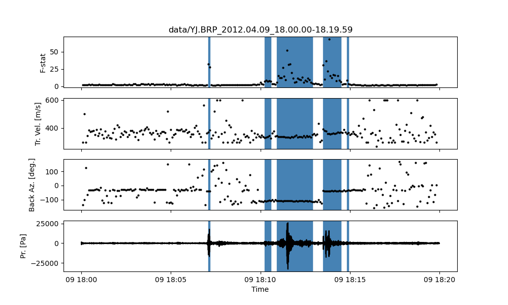
One useful feature of the detections methods in InfraPy is the ability to merge detections. By setting --merge-dets True on the command line or merge_dets = True in the configuration file, any pair of detections that are separated by less than the larger of their durations and have back azimuth differences less than the specified threshold will be combined. Re-running the detection analysis with this option turn on and comparing the results:
infrapy run_fd --config-file config/detection_local.config --local-fk-label data/YJ.BRP_2012.04.09_18.00.00-18.19.59 --merge-dets True infrapy plot fd --config-file config/detection_local.config
In some cases, the parameters in the detection analysis are modified without changing the beamforming configuration and the run_fd is useful in such scenarios to avoid repeatedly running the fk analysis. However, most of the time, the beamforming and detection analysis are run together. This can be accomplished in the InfraPy CLI via the run_fkd option.
infrapy run_fkd --config-file config/detection_local.config
This option essentially combines the run_fk and run_fd options into a single analysis run.
In addition to analysis of local data, InfraPy’s use of obspy.clients.fdsn methods enables analysis of data available on IRIS and similar FDSNs. Instead of specifying local waveform files, this requires defining the FDSN (e.g., IRIS, USGS) as well as the network, station, channel, and location information of the array. Lastly, the start and end time are also needed to identify the segment of data to download for analysis. This information can be entered on the command line, but it’s easier to simply write up a config file in most cases (recall that individual parameters can be overwritten on the command line, so the station or start/end times can be modified as needed). An example analysis from the IMS I53US array is included in examples/config/detection_fdsn.config:
[WAVEFORM IO] fdsn = IRIS network = IM station = I53* location = * channel = *DF starttime = 2018-12-19T01:00:00 endtime = 2018-12-19T03:00:00 [DETECTION IO] local_fk_label = auto local_detect_label = auto
Running this analysis will pull 2 hours of data from the International Monitoring System (IMS) I53US infrasound station from December 19th, 2018 that includes a signal produced by a bolide. Visualization can be slightly slower as the data is re-downloaded from IRIS with each use of the command line calls. This can be avoided using the write-wvfrms Utility Functions function. Due to the emergent nature of the signal, --merge-dets needs to be activated to obtain a useful result as seen below.

Although not currently accessible in the CLI methods, an FDSN station browser is available in the InfraView GUI to search for available data given a reference location, radius, and time bounds.
Analysis of data from a local database is also available through the InfraPy CLI using the Python pisces library, and is covered in a separate tutorial on Database Interfacing.

Network-Level Analyses¶

Once fk and fd analysis are run and detections are identified across a network of infrasound arrays, event identification and localization can be completed. The detection set used in the Blom et al. (2020) evaluation of a pair-based, joint-likelihood association algorithm are included as an example to demonstrate these analysis steps. Detection files are in the examples/data/Blom_etal_2020/ directory and contain detections on each of 4 regional array in the western US (see the manuscript for a full discussion of the generation of this synthetic data set). Analysis of these detections and identification of events can be completed by running:

infrapy run_assoc --local-detect-label 'data/Blom_etal2020_GJI/*' --local-event-label GJI_example --cpu-cnt 4
Note that once again quotes are needed to define multiple files for ingestion. This analysis can be on the slow side, so it’s recommended to add on a --cpu-cnt option and multithread the computation of the joint-likelihood values. For this analysis, multi-threading distributes the individual joint-likelihood calculations between pairs of detections to available threads. The analysis results will be summarized to the screen,
#####################################
##                                 ##
##             InfraPy             ##
##       Association Analysis      ##
##                                 ##
#####################################

Data summary:
  local_detect_label: data/Blom_etal2020_GJI/*
  local_event_label: example
  starttime: None
  endtime: None

Parameter summary:
  back_az_width: 10.0
  range_max: 2000.0
  resolution: 180
  distance_matrix_max: 8.0
  cluster_linkage: weighted
  cluster_threshold: 5.0
  trimming_threshold: 3.8

Loading detections from files:
        data/Blom_etal2020_GJI/NVIAR.dets.json
        data/Blom_etal2020_GJI/I57US.dets.json
        data/Blom_etal2020_GJI/DLIAR.dets.json
        data/Blom_etal2020_GJI/PDIAR.dets.json

Running event identification for: 2010-01-01T09:35:59.773Z - 2010-01-01T13:23:14.773Z
        Computing joint-likelihoods...
                Progress:       [>>>>>>>>>>>>>>>>>>>>>>>>>>>>>>>>>>>>>>>>>>>>>>>>>>]
        Clustering detections into events...
        Trimming poor linkages and repeating clustering analysis...

Running event identification for: 2010-01-01T10:51:44.773Z - 2010-01-01T14:38:59.773Z
        Computing joint-likelihoods...
                Progress:       [>>>>>>>>>>>>>>>>>>>>>>>>>>>>>>>>>>>>>>>>>>>>>>>>>>]
        Clustering detections into events...
        Trimming poor linkages and repeating clustering analysis...

Running event identification for: 2010-01-01T12:07:29.773Z - 2010-01-01T15:54:44.773Z
        Computing joint-likelihoods...
                Progress:       [>>>>>>>>>>>>>>>>>>>>>>>>>>>>>>>>>>>>>>>>>>>>>>>>>>]
        Clustering detections into events...
        Trimming poor linkages and repeating clustering analysis...

Running event identification for: 2010-01-01T13:23:14.773Z - 2010-01-01T17:10:29.773Z
        Computing joint-likelihoods...
                Progress:       [>>>>>>>>>>>>>>>>>>>>>>>>>>>>>>>>>>>>>>>>>>>>>>>>>>]
        Clustering detections into events...
        Trimming poor linkages and repeating clustering analysis...

Cleaning up and merging clusters...
identified 3 events.
The analysis breaks the detection list into segments defined by the maximum propagation distance allows in order to avoid including detections in one analysis that will not be associated with others due to differences in detection times and typical infrasonic propagation velocities. For each event identified in the analysis, a new .dets.json file is written that includes the subset of the original detections that have been identified as originating from a common event. The naming convention of these files is local_event_label_ev-#.dets.json and the example analysis here should have identified 3 events.

Detection sets can be visualized on a map using the plot dets option. This is useful in determining a useful maximum range for event identification and localization analysis. For the above analysis of the Blom et al. (2020) synthetic data set, the full data set can be visualized with,
infrapy plot dets --local-detect-label 'data/Blom_etal2020_GJI/*'
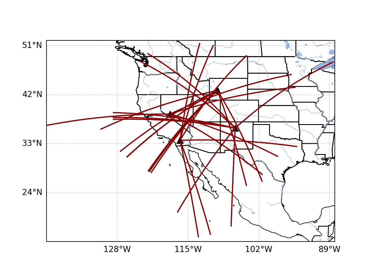
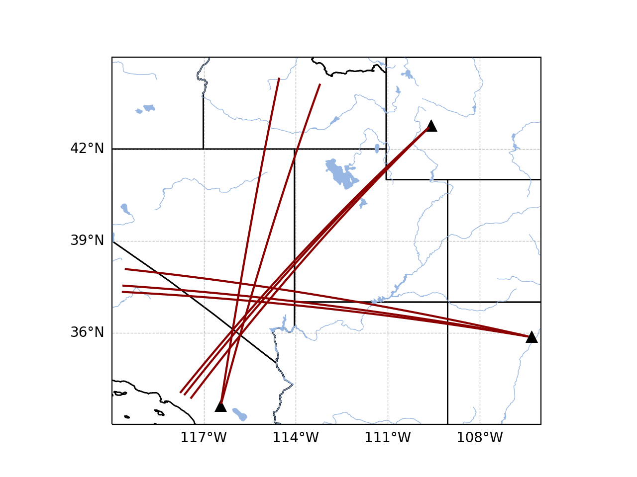
This result is rather busy, but plotting each individual event’s detections shows that the association algorithm correctly identified the events,
infrapy plot dets --local-detect-label 'GJI_example-ev0.dets.json' --range-max 1000

Once an event has been identified, the detections can be analyzed using the Bayesian Infrasonic Source Localization (BISL) methods as discussed in Blom et al. (2015). This requires specifying the detection list file as well as an output location file label,

infrapy run_loc --local-detect-label GJI_example-ev0  --local-loc-label GJI_example-ev0

The analysis steps are updated as localization is performed and the resulting location and origin time information is printed to screen as well as written into an output file (the output file for InfraPy’s localization is also a .json format file, but it’s naming convention uses “.loc.json” to distinguish it from a “.dets.json” detection file)

#####################################
##                                 ##
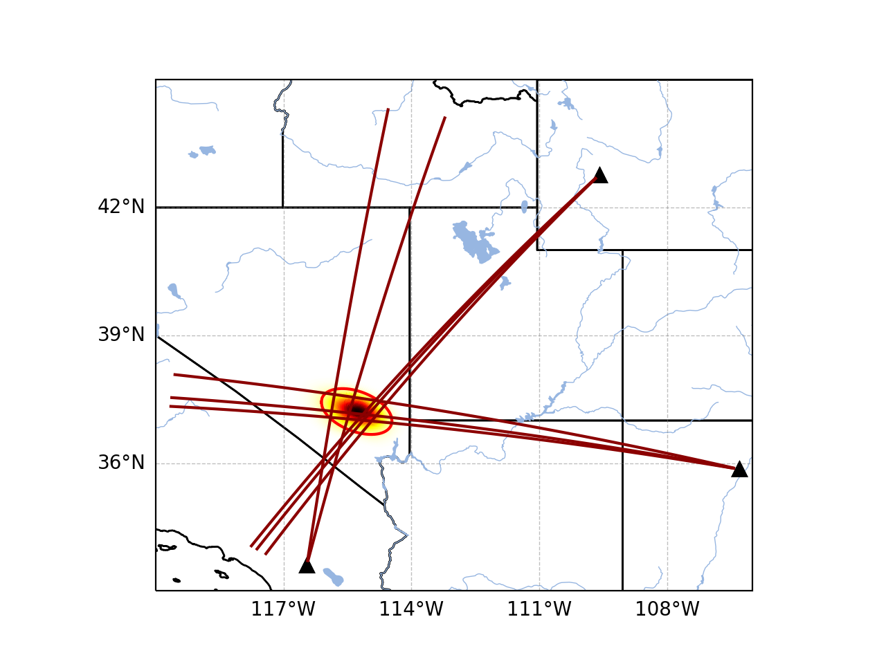
##             InfraPy             ##
##      Localization Analysis      ##
##                                 ##
#####################################

Data summary:
  local_event_label: example1-ev0
  local_loc_label: example1-ev0

Parameter summary:
  back_az_width: 10.0
  range_max: 2000.0
  resolution: 180
  src_est: None
  pgm_file: None

Loading detections from file: example1-ev0.dets.json

Running Bayesian Infrasonic Source Localization (BISL) Analysis...
        Identifying integration region...
        Computing marginalized spatial PDF...
        Computing confidence ellipse parameters...
        Computing marginalized origin time PDF...

BISL Summary:
Maximum a posteriori analysis:
        Source location: 37.212, -115.283
        Source time: 2010-01-01T12:11:16.645000
Source location analysis:
        Latitude (mean and standard deviation): 37.212 +/- 27.882 km.
        Longitude (mean and standard deviation): -115.283 +/- 34.18 km.
        Covariance: -0.41.
        Area of 95 confidence ellipse: 17938.387 square kilometers
Source time analysis:
        Mean and standard deviation: 2010-01-01T12:11:55.838 +/- 100.512 second
        Exact 90% confidence bounds: [2010-01-01T12:09:12.885, 2010-01-01T12:14:46.185]

Writing localization result into GJI_example-ev0.loc.json

The localization result can be visualized in a number of ways. Firstly, the detecting arrays and location estimate can be plotted on map using,

infrapy plot loc --local-detect-label GJI_example-ev0 --local-loc-label GJI_example-ev0 --range-max 1200.0

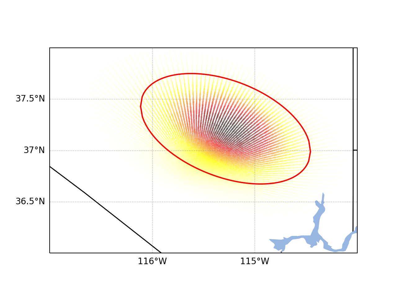
For visualization of the source region in more detail, the --zoom option can be set to true and the map zooms in to show only the estimated source region.

infrapy plot loc --local-detect-label GJI_example-ev0 --local-loc-label GJI_example-ev0 --zoom true

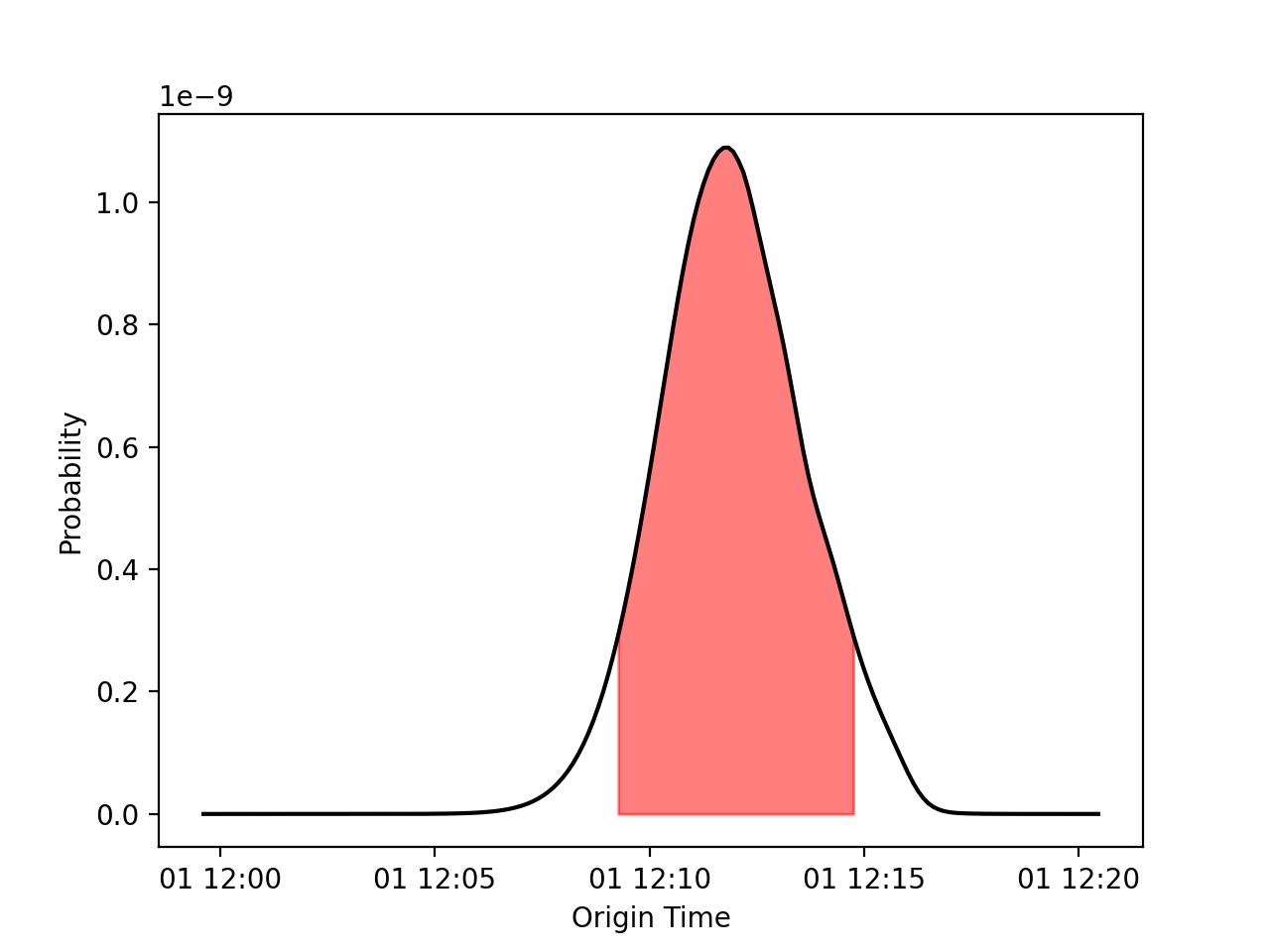
Lastly, the origin time is estimated as part of the BISL analysis and can be visualized as,

infrapy plot origin-time --local-loc-label GJI_example-ev0

For above-ground explosive sources for which source models such as the Kinney & Graham blastwave scaling laws can be used to relate acoustic power to yield, InfraPy’s Spectral Yield Estimate (SpYE) methods can be applied. Usage of these methods requires a detection file, waveform data for detecting stations, and transmission loss models relating downrange observations to a near-source reference point. Analysis of the Humming Roadrunner 5 event is included (requires downloading the separate infrapy-data repository):
infrapy run_yield --local-wvfrms '../infrapy-data/hrr-5/*/*.sac' --local-detect-label data/HRR-5.dets.json --src-lat 33.5377 --src-lon -106.333961 --tlm-label "../infrapy/propagation/priors/tloss/2007_08-" --local-yld-label "HRR-5"
As with other analysis methods, parameter information will be summarized and high level results:

The example here utilizes a ground truth location for the source; though, the method can also accept a location result file from BISL ([...].loc.json) and extract the location from that source. The current implementation can only utilize locally saved waveform data ingested as a single large stream and sub-divided using the network and station info in the detection file. Eventually, it is planned to allow the methods to pull from an FDSN or database, but for now analysis requires pulling waveform files (this can be done using infrapy utils write-wvfrms).

Visualization of the SpYE analysis result can be done by referencing the output file,
infrapy plot yield --local-yld-label "HRR-5"
This once again prints the MaP yield and confidence bounds and produces a figure such as that shown below where the left panel shows the PDF for yield and the right panel shows the predicted spectral amplitude near the source (specifically at a stand off distance of --ref-rng).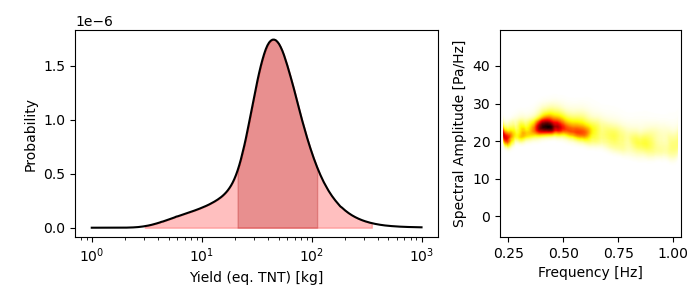

Scripting and Notebook-Based Analysis¶

In addition to the command line interface methods for infrapy, the analysis algorithms can be imported directly into user Python scripts or notebooks for custom applications. Example import and usage scripts are included in the examples/ directory and will be detailed below for this somewhat more advanced usage. The example scripts are summarized in the below table.

example_fkd.py	Run beamforming and detection analysis on an Obspy stream
example_assoc.py	Run event identification methods on a list of detections
example_bisl.py	Run localization methods on a list of detections
example_yield.py	Run spectral yield estimation methods

The beamforming and detection analysis can be imported from the infrapy.detection.beamforming_new library. Beamforming analysis includes setting up an ObsPy stream, converting it to an array data instance, and then scanning through with a defined analysis window.

import numpy as np

from obspy.core import read
from infrapy.detection import beamforming_new

if __name__ == '__main__':

    # ######################### #
    #     Define Parameters     #
    # ######################### #
    sac_glob = "data/YJ.BRP*.SAC"

    freq_min, freq_max = 0.5, 2.5
    fk_win_len, window_step = 10.0, 2.5
    sig_start, sig_end = 600, 800

    back_az_vals = np.arange(-180.0, 180.0, 2.0)
    trc_vel_vals = np.arange(300.0, 600.0, 2.5)

    # ######################### #
    #        Run Methods        #
    # ######################### #

    # Read data and convert to array format
    x, t, t0, geom = beamforming_new.stream_to_array_data(read(sac_glob))
    M, N = x.shape

    # Define slowness and delays
    slowness = beamforming_new.build_slowness(back_az_vals, trc_vel_vals)
    delays = beamforming_new.compute_delays(geom, slowness)

    # Run beamforming in each window and find best beam info
    times, beam_results = [],[]
    for window_start in np.arange(sig_start, sig_end, window_step):
        if window_start + fk_win_len > sig_end:
            break

        X, S, f = beamforming_new.fft_array_data(x, t, window=[window_start, window_start + fk_win_len])
        beam_power = beamforming_new.run(X, S, f, geom, delays, [freq_min, freq_max])
        peaks = beamforming_new.find_peaks(beam_power, back_az_vals, trc_vel_vals)

        times = times + [[t0 + np.timedelta64(int(window_start), 's')]]
        beam_results = beam_results + [[peaks[0][0], peaks[0][1], peaks[0][2] / (1.0 - peaks[0][2]) * (x.shape[0] - 1)]]

    times = np.array(times)[:, 0]
    beam_results = np.array(beam_results)

Detection analysis is then completed by scanning back through the beamforming results and can be appended to the end of the above beamforming analysis as it requires the times and beam_results information computed there.

fd_win_len = 60 * 5
det_thresh = 0.99

min_seq = 5
back_az_lim = 10

TB_prod = (freq_max - freq_min) * fk_window_len
dets = beamforming_new.detect_signals(times, beam_results, fd_win_len, TB_prod, M, min_seq=min_seq, back_az_lim=back_az_lim)

for det in dets:
    print("Detection time:", det[0], '\t', "Rel. detection onset:", det[1], '\t',"Rel. detection end:", det[2], '\t',end=' ')
    print("Back azimuth:", np.round(det[3], 2), '\t', "Trace velocity:", np.round(det[4], 2), '\t', "F-stat:", np.round(det[5], 2), '\t', "Array dim:", M)

The association methods require ingesting a detection list and defining a clustering threshold for the hierarchical linkage cut off. The likelihood methods include a function to read in a .json format file as output in the CLI detection analysis.

from infrapy.association import hjl
from infrapy.utils import data_io

if __name__ == '__main__':
    det_list = data_io.json_to_detection_list('data/example1.dets.json')
    clustering_threshold = 5.0

    labels, dists = hjl.run(det_list, clustering_threshold)

    clusters, qualities = hjl.summarize_clusters(labels, dists)
    for n in range(len(clusters)):
        print("Cluster:", clusters[n], '\t', "Cluster Quality:", 10.0**(-qualities[n]))

Similar to the association methods, localization requires just a detection set from an event:

from infrapy.location import bisl
from infrapy.utils import data_io

if __name__ == '__main__':
    det_list = data_io.json_to_detection_list('data/example2.dets.json')

    result,pdf = bisl.run(det_list)
    print(bisl.summarize(result))

Yield estimation analysis is a bit challenging to perform interactively or even in an automated way because analysis parameters include the detection file for the event, waveform data from the various detecting stations, transmission loss models, and a source model. An initial version of this is implemented as part of InfraPy’s command line interface as discussed above; however, it is likely a user may prefer to interact directly with the data ingestion and analysis.

from obspy.core import read

import numpy as np

import matplotlib.pyplot as plt

from infrapy.utils import data_io
from infrapy.propagation import infrasound

from infrapy.characterization import spye

if __name__ == '__main__':
    # ######################### #
    #     Define Parameters     #
    # ######################### #

    det_file = "data/HRR-5.dets.json"
    wvfrm_path = "../infrapy-data/hrr-5/*/*.sac"
    tloss_path = "../infrapy/propagation/priors/tloss/2007_08-"

The analysis parameters include a noise option (“pre” or “post” detection window), a window buffer factor that extends the sample window beyond the detection window by some factor (0.2 meaning a 20% increase in the window length here), a source location, frequency band, yield range, and reference distance from the source at which to compute the source spectral estimate. If a ground truth yield is known it can be specified and the frequency-yield resolution of the grid can be specified.

ns_opt = "post"
win_buffer = 0.2

src_loc = np.array([33.5377, -106.333961])
freq_band = np.array([0.25, 2.0])
yld_rng = np.array([1.0e3, 1000.0e3])
ref_rng = 1.0

grnd_truth=None
resol = 200

The detection list and waveform files are ingested and spectral amplitudes are computed,

# ############################# #
#     Define the detections     #
#          and spectra          #
# ############################# #
det_list = data_io.json_to_detection_list(det_file)
st_list = [Stream([tr for tr in read(wvfrm_path) if det.station in tr.stats.station]) for det in det_list]
smn_specs = spye.extract_spectra(det_list, st_list, win_buffer=win_buffer, ns_opt=ns_opt)

The transmission loss model models are defined and loaded,

# ######################### #
#     Load TLoss Models     #
# ######################### #
tloss_f_min, tloss_f_max, tloss_f_cnt = 0.025, 2.5, 25

models = [0] * 2
models[0] = list(np.logspace(np.log10(tloss_f_min), np.log10(tloss_f_max), tloss_f_cnt))
models[1] = [0] * tloss_f_cnt
for n in range(tloss_f_cnt):
    models[1][n] = infrasound.TLossModel()
    models[1][n].load(tloss_path + "%.3f" % models[0][n] + "Hz.pri")

Finally, analysis can be performed, and results printed and visualized,

# ######################## #
#         Run Yield        #
#    Estimation Methods    #
# ######################## #
yld_results = spye.run(det_list, smn_specs, src_loc, freq_band, models, yld_rng=yld_rng, ref_src_rng=ref_rng, resol=resol)

print('\nResults:')
print('\t' + "Maximum a Posteriori Yield:", yld_results['yld_vals'][np.argmax(yld_results['yld_pdf'])])
print('\t' + "68% Confidence Bounds:", yld_results['conf_bnds'][0])
print('\t' + "95% Confidence Bounds:", yld_results['conf_bnds'][1])

plt.semilogx(yld_results['yld_vals'], yld_results['yld_pdf'])
plt.fill_between(yld_results['yld_vals'], yld_results['yld_pdf'], where=np.logical_and(yld_results['conf_bnds'][0][0] <= yld_results['yld_vals'], yld_results['yld_vals'] <= yld_results['conf_bnds'][0][1]), color='g', alpha=0.25)
plt.fill_between(yld_results['yld_vals'], yld_results['yld_pdf'], where=np.logical_and(yld_results['conf_bnds'][1][0] <= yld_results['yld_vals'], yld_results['yld_vals'] <= yld_results['conf_bnds'][1][1]), color='g', alpha=0.25)

plt.show()